Image Classfication
- Home
- Image Classfication
Table of Contents:
Motivation. Assigning an input image one label from a fixed set of categories. This is one of the core problems in Computer Vision.
Challenges.
Data-driven approach. : Provide the computer with many examples of each class and then develop learning algorithms that look at these examples and learn about the visual appearance of each class. This approach is referred to as a data-driven approach, since it relies on first accumulating a training dataset of labeled images.
The image classification pipeline.
As our first approach, we will develop what we call a Nearest Neighbor Classifier. This classifier has nothing to do with Convolutional Neural Networks and it is very rarely used in practice, but it will allow us to get an idea about the basic approach to an image classification problem.
Suppose now that we are given the CIFAR-10 training set of 50,000 images (5,000 images for every one of the labels), and we wish to label the remaining 10,000. The nearest neighbor classifier will take a test image, compare it to every single one of the training images, and predict the label of the closest training image.
Given two images and representing them as vectors $( I_1, I_2 )$ , a reasonable choice for comparing them might be the L1 distance:
Where the sum is taken over all pixels. Here is the procedure visualized:
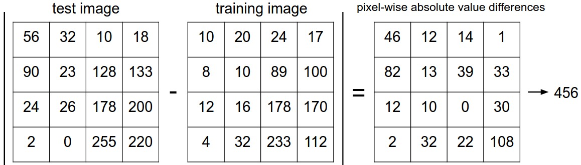
Notice that as an evaluation criterion, it is common to use the accuracy, which measures the fraction of predictions that were correct. Notice that all classifiers we will build satisfy this one common API: they have a train(X,y) function that takes the data and the labels to learn from. Internally, the class should build some kind of model of the labels and how they can be predicted from the data. And then there is a predict(X) function, which takes new data and predicts the labels. Of course, we've left out the meat of things - the actual classifier itself. Here is an implementation of a simple Nearest Neighbor classifier with the L1 distance that satisfies this template:
import numpy as np

                        class NearestNeighbor(object):
                        def __init__(self):
                        pass

                        def train(self, X, y):
                        """ X is N x D where each row is an example. Y is 1-dimension of size N """
                        # the nearest neighbor classifier simply remembers all the training data
                        self.Xtr = X
                        self.ytr = y

                        def predict(self, X):
                        """ X is N x D where each row is an example we wish to predict label for """
                        num_test = X.shape[0]
                        # lets make sure that the output type matches the input type
                        Ypred = np.zeros(num_test, dtype = self.ytr.dtype)

                        # loop over all test rows
                        for i in range(num_test):
                        # find the nearest training image to the i'th test image
                        # using the L1 distance (sum of absolute value differences)
                        distances = np.sum(np.abs(self.Xtr - X[i,:]), axis = 1)
                        min_index = np.argmin(distances) # get the index with smallest distance
                        Ypred[i] = self.ytr[min_index] # predict the label of the nearest example

                        return Ypred
There are many other ways of computing distances between vectors. Another common choice could be to instead use the L2 distance, which has the geometric interpretation of computing the Euclidean distance between two vectors. The distance takes the form:
In other words we would be computing the pixelwise difference as before, but this time we square all of them, add them up and finally take the square root. In numpy, using the code from above we would need to only replace a single line of code. The line that computes the distances:
distances = np.sqrt(np.sum(np.square(self.Xtr - X[i,:]), axis = 1))
Note that I included the np.sqrt call above, but in a practical nearest neighbor application we could leave out the square root operation because square root is a monotonic function. That is, it scales the absolute sizes of the distances but it preserves the ordering, so the nearest neighbors with or without it are identical. If you ran the Nearest Neighbor classifier on CIFAR-10 with this distance, you would obtain 35.4% accuracy (slightly lower than our L1 distance result).
L1 vs. L2. It is interesting to consider differences between the two metrics. In particular, the L2 distance is much more unforgiving than the L1 distance when it comes to differences between two vectors. That is, the L2 distance prefers many medium disagreements to one big one. L1 and L2 distances (or equivalently the L1/L2 norms of the differences between a pair of images) are the most commonly used special cases of a p-norm.
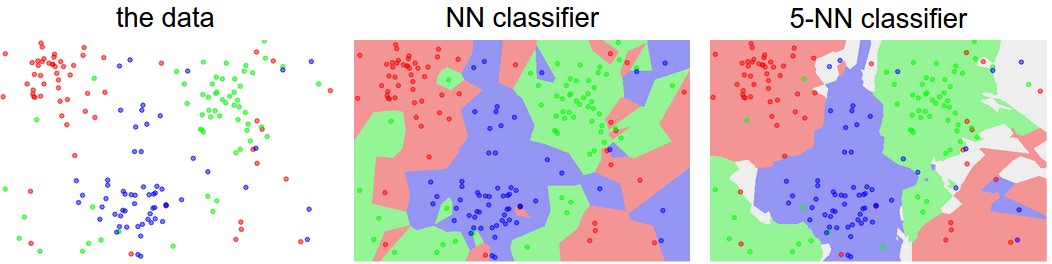
You may have noticed that it is strange to only use the label of the nearest image when we wish to make a prediction. Indeed, it is almost always the case that one can do better by using what's called a k-Nearest Neighbor Classifier. The idea is very simple: instead of finding the single closest image in the training set, we will find the top k closest images, and have them vote on the label of the test image. In particular, when k = 1, we recover the Nearest Neighbor classifier. Intuitively, higher values of k have a smoothing effect that makes the classifier more resistant to outliers:
In practice, you will almost always want to use k-Nearest Neighbor. But what value of k should you use? We turn to this problem next.
The k-nearest neighbor classifier requires a setting for k. But what number works best? Additionally, we saw that there are many different distance functions we could have used: L1 norm, L2 norm, there are many other choices we didn't even consider (e.g. dot products). These choices are called hyperparameters and they come up very often in the design of many Machine Learning algorithms that learn from data. It's often not obvious what values/settings one should choose.
You might be tempted to suggest that we should try out many different values and see what works best. That is a fine idea and that's indeed what we will do, but this must be done very carefully. In particular, we cannot use the test set for the purpose of tweaking hyperparameters. Whenever you're designing Machine Learning algorithms, you should think of the test set as a very precious resource that should ideally never be touched until one time at the very end. Otherwise, the very real danger is that you may tune your hyperparameters to work well on the test set, but if you were to deploy your model you could see a significantly reduced performance. In practice, we would say that you overfit to the test set. Another way of looking at it is that if you tune your hyperparameters on the test set, you are effectively using the test set as the training set, and therefore the performance you achieve on it will be too optimistic with respect to what you might actually observe when you deploy your model. But if you only use the test set once at end, it remains a good proxy for measuring the generalization of your classifier (we will see much more discussion surrounding generalization later in the class).
Evaluate on the test set only a single time, at the very end.
Luckily, there is a correct way of tuning the hyperparameters and it does not touch the test set at all. The idea is to split our training set in two: a slightly smaller training set, and what we call a validation set. Using CIFAR-10 as an example, we could for example use 49,000 of the training images for training, and leave 1,000 aside for validation. This validation set is essentially used as a fake test set to tune the hyper-parameters.
Here is what this might look like in the case of CIFAR-10:
# assume we have Xtr_rows, Ytr, Xte_rows, Yte as before
                    # recall Xtr_rows is 50,000 x 3072 matrix
                    Xval_rows = Xtr_rows[:1000, :] # take first 1000 for validation
                    Yval = Ytr[:1000]
                    Xtr_rows = Xtr_rows[1000:, :] # keep last 49,000 for train
                    Ytr = Ytr[1000:]

                    # find hyperparameters that work best on the validation set
                    validation_accuracies = []
                    for k in [1, 3, 5, 10, 20, 50, 100]:

                    # use a particular value of k and evaluation on validation data
                    nn = NearestNeighbor()
                    nn.train(Xtr_rows, Ytr)
                    # here we assume a modified NearestNeighbor class that can take a k as input
                    Yval_predict = nn.predict(Xval_rows, k = k)
                    acc = np.mean(Yval_predict == Yval)
                    print 'accuracy: %f' % (acc,)

                    # keep track of what works on the validation set
                    validation_accuracies.append((k, acc))
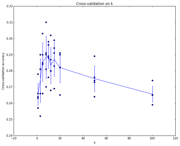
By the end of this procedure, we could plot a graph that shows which values of k work best. We would then stick with this value and evaluate once on the actual test set.
Split your training set into training set and a validation set. Use validation set to tune all hyperparameters. At the end run a single time on the test set and report performance.
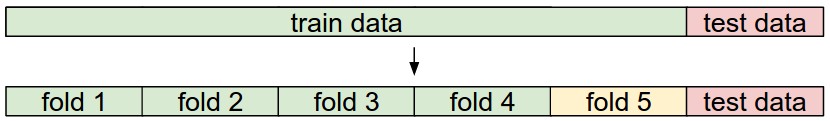
In cases where the size of your training data (and therefore also the validation data) might be small, people sometimes use a more sophisticated technique for hyperparameter tuning called cross-validation. Working with our previous example, the idea is that instead of arbitrarily picking the first 1000 datapoints to be the validation set and rest training set, you can get a better and less noisy estimate of how well a certain value of k works by iterating over different validation sets and averaging the performance across these. For example, in 5-fold cross-validation, we would split the training data into 5 equal folds, use 4 of them for training, and 1 for validation. We would then iterate over which fold is the validation fold, evaluate the performance, and finally average the performance across the different folds.
In practice. In practice, people prefer to avoid cross-validation in favor of having a single validation split, since cross-validation can be computationally expensive. The splits people tend to use is between 50%-90% of the training data for training and rest for validation. However, this depends on multiple factors: For example if the number of hyperparameters is large you may prefer to use bigger validation splits. If the number of examples in the validation set is small (perhaps only a few hundred or so), it is safer to use cross-validation. Typical number of folds you can see in practice would be 3-fold, 5-fold or 10-fold cross-validation.
Pros:
Cons:
In summary:
In next lectures we will embark on addressing these challenges and eventually arrive at solutions that give 90% accuracies, allow us to completely discard the training set once learning is complete, and they will allow us to evaluate a test image in less than a millisecond.
If you wish to apply kNN in practice (hopefully not on images, or perhaps as only a baseline) proceed as follows:
Here are some (optional) links you may find interesting for further reading:
A Few Useful Things to Know about Machine Learning, where especially section 6 is related but the whole paper is a warmly recommended reading.
Recognizing and Learning Object Categories, a short course of object categorization at ICCV 2005.